I primarly wrote this to test .md formatting on this website.

Transformer architecture was first introduced in the now famous "Attention Is All You Need" paper in 2017. The main goal of transformer is to model long-range dependencies in sequences through parallelization of matrix operations.

Before transformer, the field of processing and generating text by Neural nets relied on processing tokens sequentially: $h_t = f(x_t, h_{t-1})$. For sequence e.g. "Car has four wheels.", when processing the token "four", $x_t$ is its embedding vector, and $h_{t-1}$ is a latent representation summarizing the "Car has". $f$ (e.g. an LSTM cell) integrates the new input $x_t$ with prior hidden state $h_{t-1}$ to produce $h_t$, a (compressed) representation of "Car has four". The obvious problem is than each token is processed sequentially (token 1 -> token 2 -> token 3....), which heavily restricts the computation. Another, major issue, which I will jsut mention and not explain to detail, is the problem with vanishing/exploding gradients during training and context loss over long sequences - at each time step $t$ the entire previous representation is compressed into a fixed size vector $h_t$...

As mentioned, transformer architecture eliminates recurrence and instead computes relationships between all tokens in parallel using process called self attention. But let's start from begging.

Input

The input to an transformer is a sequence of tokens $X \in \mathbb{R}^{n \times d}$ ($n$ is the seq. length and $d$ is the embedding dimension). The model treats input as a set not an ordered sequence - permutation-invariant, thus it uses Positional Encoding using sinusoidal functions to inject order of tokens in sequence:

$$\begin{aligned} PE_{pos,,2i} &= \sin!\left(\frac{pos}{10000^{2i/d}}\right) \ \ PE_{pos,,2i+1} &= \cos!\left(\frac{pos}{10000^{2i/d}}\right) \ \ z_t &= x_t + PE_t \end{aligned}$$

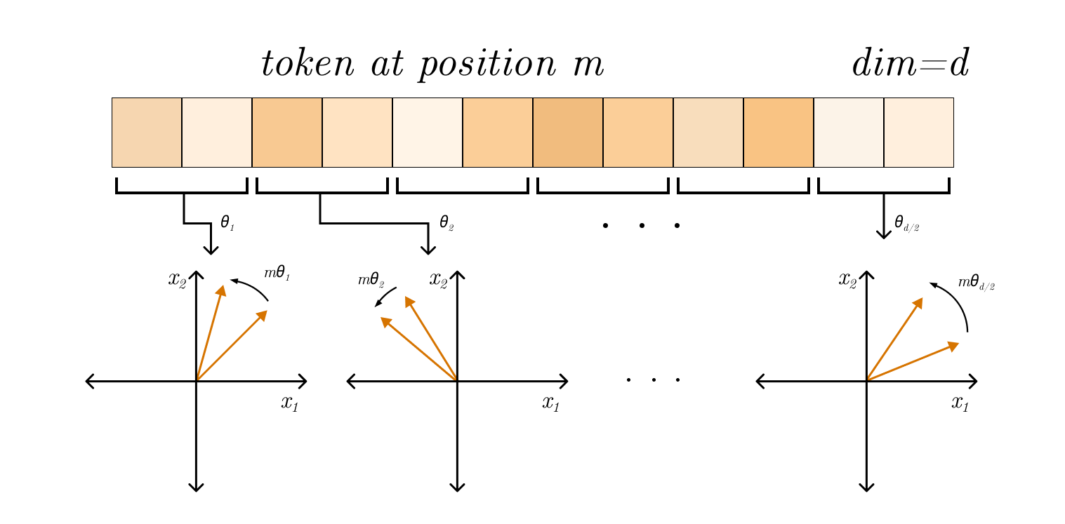
In other terms, instead of attaching indices tokens, the transformer gets a unique vector in $\mathbb{R}^d$. Using sinusoidal encoding also implies that: $$PE_{t+k} = A_kPE_t$$ for some linear transformation $A_k$ enabling the model to infer relative distances. Last but not least, the fact that the pos. encodings are deterministic and not learned helps generalize the model.

$X$ is projected into spaces: $$\begin{aligned} Q = XW_Q, \quad K=XW_K, \quad V=XW_V \ \ \text{where} \quad W_Q, W_K, W_V \in \mathbb{R^{d\times d_k}} \ \ \text{which means} \quad Q,K,V \in \mathbb{R^{n\times d_k}} \end{aligned}$$

Attention

At high level, attention allows each token to look at all other tokens, score their relevance and builds a weighted combination.
Let's lay it out on the table, the main (famous) equation of scaled dot-product attention: $$\boxed{ \begin{aligned} A = \text{softmax}\left(\frac{QK^T}{\sqrt{d_k}}\right)V \ \text{Attention}(Q,K,V) = AV \end{aligned} }$$ Looking at this attention equation, the numerator: $S =QK^T \in \mathbb{R}^{n\times n}$ where each $S_{ij} = \langle q_i, k_j\rangle$ tells us how well token $i$ matches token $j$ in the learned representation space. In higher level terms, larger $S_{ij}$ means that token $j$ is more relevant to token $i$ and vice versa. The $\sqrt{d_k}$ is introduced to stabilize training as products grow with $d_k$ which could push gradients near zero (softmax saturation).

The softmax function $softmax: \mathbb{R}^K \rightarrow (0,1)^K$ where $K>1$ in its general form: $$softmax(z)$$i = \frac{e^{z_i}}{\sum{j=1}^Ne^{z_j}} where $z = (z_1, \dots, z_K)\in \mathbb{R}^K$ and computes each component of $softmax(\textbf{z})\in (0,1)^K$. For our attention case, this means: $$A_{ij} = \frac{exp(S_{ij}/\sqrt(d_k))}{\sum_{j'=1}^N exp(S_{ij'}/\sqrt(d_k))}$$ This guarantees that $A_{ij}>0 \land \sum_j A_{ij} = 1$ and each row $A_i$ therefore shows how token $i$ distributes its attention across the entire input sequence. This builds a matrix $A$, where each row $A_i$ is a probability distribution over tokens, thus: $$\text{out}$$i = \sum{j=1}^n{A_{ij}v_j} is a contextual embedding of token $i$. Instead of utilizing just single attention for the entire sequence, the model learns several token2token pairs at once in parallel using Multi Head Attention: $$\begin{aligned} head_h = Attention(XW_Q^{(h)},XW_K^{(h)},XW_V^{(h)}) \ \ MHA(X) = Concat(head_1, \dots, head_H)W_0 \end{aligned}$$

Transformer Block

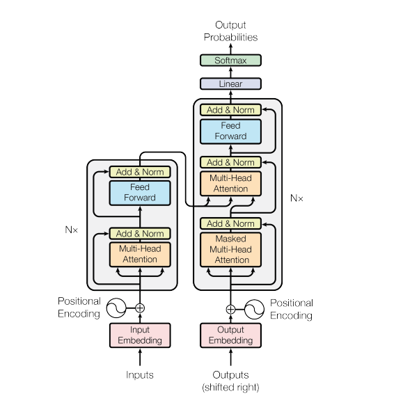
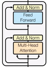
A full transformer layer consist of:

Firstly MHA is computed, than residual connection (Add) is applied to it $X + MHA(X)$ to preserve information: each layer updates the representation. Afterwards normalization function is used for stable distribution via: $$LayerNorm(y_i)=\gamma \odot \frac{y_i - \mu_i}{\sqrt{\sigma_i^2+\epsilon}}+\beta$$ where $\gamma$(scale) and $\beta$(shift/bias) are learned. Next, the Feedforward Network introduces non-linearity ($\sigma$) via $FFN(x) = \sigma(xW_1 + b1)W_2 + b_2$ where the goal is that $W_1$ expands the features, $\sigma$ transformers them and $W_2$ compresses them back into correct representation.

Encoder & Decoder

As visible on the full architecture above, transformer is divided into Encoder and Decoder sections. The encoder produces a set of contextual representations $H = (h_1, \dots h_n)$. The decoder than generates the output autoregressively: $y_t$ is conditioned on prev. generated $y_{<t}$ and encoded input $H$. A mechanism called CrossAttention(Q,K,V) enables it, where $Q$ comes from decoder states and $K, V$ come from encoder output $H$. I asked LLM on this to produced an analogy, and it generated quite an intuitive one:

Encoder is like a court that builds a complete, structured case file from all evidence; decoder is a lawyer writing the final argument, repeatedly checking that case file to pick the most relevant facts while composing each sentence. (Unspecified AI, 2026)

Code

The following code is an implementation of transformer architecture from scratch in NumPy.